kmeans

K-means in a “toy” dataset

Lets construct a more small but instructive example:

X = c(7, 3, 1, 5, 1, 7, 8, 5)
Y = c(1, 4, 5, 8, 3, 8, 2, 9)
rnames = c("x1", "x2", "x3", "x4", "x5", "x6", "x7", "x8")
kdata = data.frame(X, Y, row.names = rnames)

and plot the 2D dataset:

plot(kdata, pch = 15)
text(kdata, labels = row.names(kdata), pos = 2)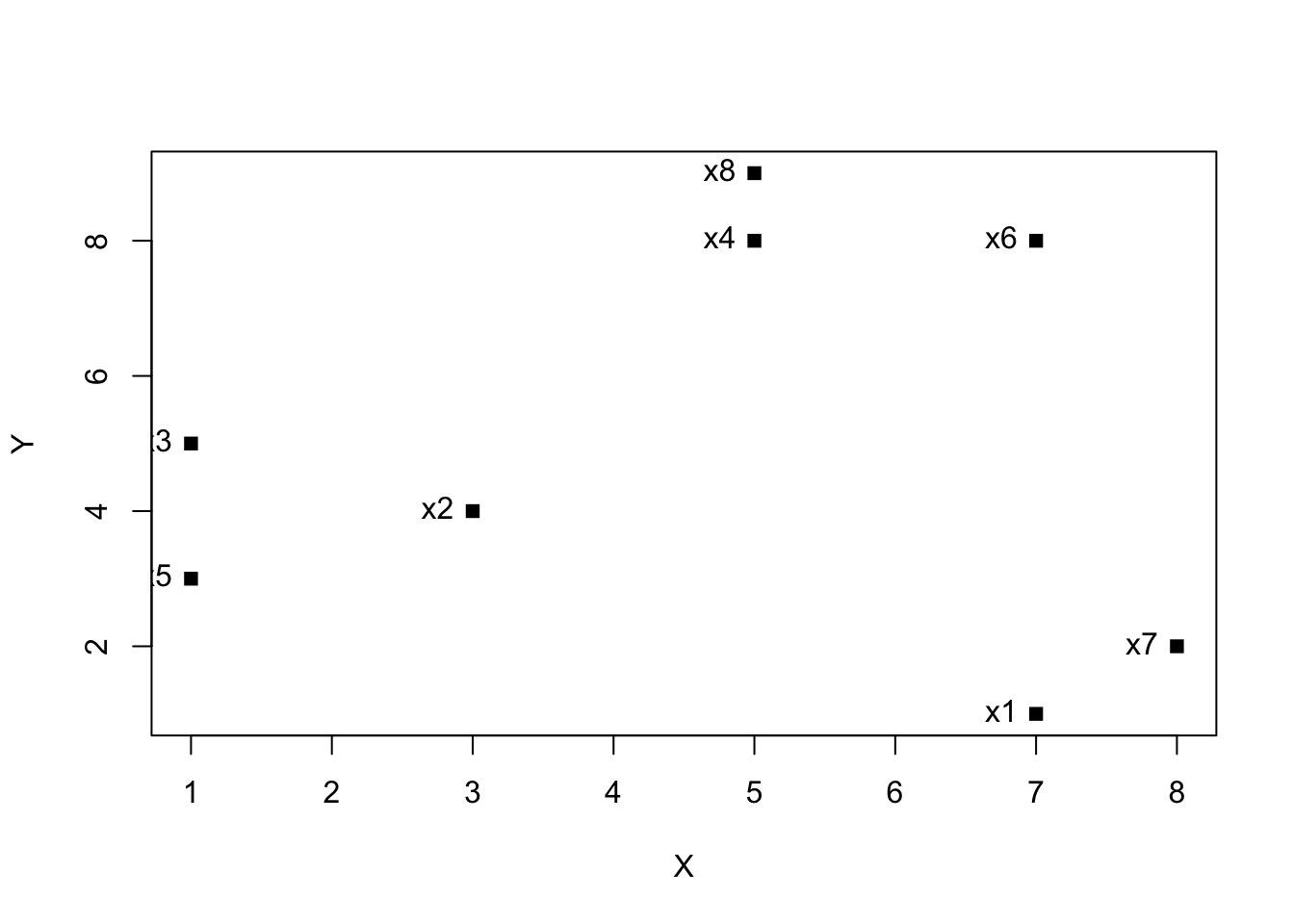

Create the clustering

# we take as initial centers the first 3 points and this implies also that k = 3
clust = kmeans(kdata, centers=kdata[1:3,])
clust$centers

##          X        Y
## 1 7.500000 1.500000
## 2 5.666667 8.333333
## 3 1.666667 4.000000

clust$cluster

## x1 x2 x3 x4 x5 x6 x7 x8 
##  1  3  3  2  3  2  1  2

we can also easily retrieve metrics like cohesion and separation.

cohesion = clust$tot.withinss
separation = clust$betweenss

and make a nice visualization

plot(kdata, col = clust$cluster, pch = 15)
text(kdata, labels = row.names(kdata), pos = 2)
points(clust$centers, col = 1:length(clust$centers), pch = "+", cex = 2)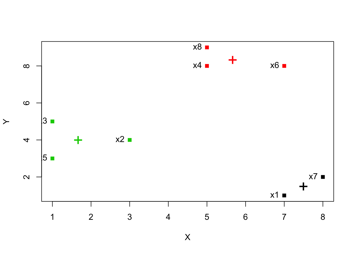

K-means for the iris dataset

Lets apply the k-means clustering algorithm to the iris dataset. To begin with, we will exclude the Species column.

data <- iris[,-5]
clustering = kmeans(data, centers = 3)
clustering

## K-means clustering with 3 clusters of sizes 62, 38, 50
## 
## Cluster means:
##   Sepal.Length Sepal.Width Petal.Length Petal.Width
## 1     5.901613    2.748387     4.393548    1.433871
## 2     6.850000    3.073684     5.742105    2.071053
## 3     5.006000    3.428000     1.462000    0.246000
## 
## Clustering vector:
##   [1] 3 3 3 3 3 3 3 3 3 3 3 3 3 3 3 3 3 3 3 3 3 3 3 3 3 3 3 3 3 3 3 3 3 3 3
##  [36] 3 3 3 3 3 3 3 3 3 3 3 3 3 3 3 1 1 2 1 1 1 1 1 1 1 1 1 1 1 1 1 1 1 1 1
##  [71] 1 1 1 1 1 1 1 2 1 1 1 1 1 1 1 1 1 1 1 1 1 1 1 1 1 1 1 1 1 1 2 1 2 2 2
## [106] 2 1 2 2 2 2 2 2 1 1 2 2 2 2 1 2 1 2 1 2 2 1 1 2 2 2 2 2 1 2 2 2 2 1 2
## [141] 2 2 1 2 2 2 1 2 2 1
## 
## Within cluster sum of squares by cluster:
## [1] 39.82097 23.87947 15.15100
##  (between_SS / total_SS =  88.4 %)
## 
## Available components:
## 
## [1] "cluster"      "centers"      "totss"        "withinss"    
## [5] "tot.withinss" "betweenss"    "size"         "iter"        
## [9] "ifault"

The clustering object contains a lot of informations and components:

The number of clusters (3) and their sizes
The centers of the 3 clusters
The clustering vector denoting which speciment (row) belongs to which cluster
The sum of squares of the distance between points and their centers for every cluster
- total_SS is the sum of squared distances of each data point to the global sample mean
- between_SS is the total_SS minus the the sum of the sum of square distances between points and their centers
- The ratio will be close to 0 (0%) if there is no discernible pattern and closer to 1 (100%) if there is.
and other components like:

# The centers
clustering$centers

##   Sepal.Length Sepal.Width Petal.Length Petal.Width
## 1     5.901613    2.748387     4.393548    1.433871
## 2     6.850000    3.073684     5.742105    2.071053
## 3     5.006000    3.428000     1.462000    0.246000

# The clustering
clustering$cluster

##   [1] 3 3 3 3 3 3 3 3 3 3 3 3 3 3 3 3 3 3 3 3 3 3 3 3 3 3 3 3 3 3 3 3 3 3 3
##  [36] 3 3 3 3 3 3 3 3 3 3 3 3 3 3 3 1 1 2 1 1 1 1 1 1 1 1 1 1 1 1 1 1 1 1 1
##  [71] 1 1 1 1 1 1 1 2 1 1 1 1 1 1 1 1 1 1 1 1 1 1 1 1 1 1 1 1 1 1 2 1 2 2 2
## [106] 2 1 2 2 2 2 2 2 1 1 2 2 2 2 1 2 1 2 1 2 2 1 1 2 2 2 2 2 1 2 2 2 2 1 2
## [141] 2 2 1 2 2 2 1 2 2 1

# The total sum of squares (the sum of squared distances of each data point to the global sample mean)
clustering$totss

## [1] 681.3706

# The per cluster sum of squares
clustering$withinss

## [1] 39.82097 23.87947 15.15100

# The sum of per cluster sum of squares
clustering$tot.withinss

## [1] 78.85144

# The total sum of squares minus the sum of per cluster sum of squares
clustering$betweenss

## [1] 602.5192

# The sizes of the clusters
clustering$size

## [1] 62 38 50

# The number of iterations before conversion
clustering$iter

## [1] 2

# Integer indicating possible algorithm problem
clustering$ifault

## [1] 0

Comparing cluster to classes

For comparing the groupings provided by k-means with the actual classes we can use the table function:

table(iris$Species, clustering$cluster)

##             
##               1  2  3
##   setosa      0  0 50
##   versicolor 48  2  0
##   virginica  14 36  0

With different initial centers in k-means one will get different values in the table above.

Plotting

Lets also plot 2 dimensions of the iris dataset and visualize the clusters and their centers:

plot(iris[c("Sepal.Length", "Sepal.Width")], col = clustering$cluster)
points(clustering$centers[,c("Sepal.Length", "Sepal.Width")], col = 1:3, pch = 8, cex=2)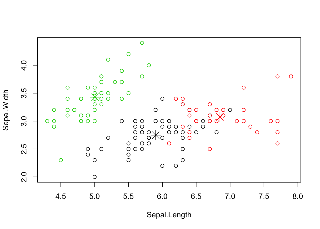

Selecting number of clusters

Returning to the iris dataset, a technique to find the number of clusters that describe the data better we can calculate the SSE (Sum of Squared Errors) for different number of clusters, say k = 1, 2, …, 10 etc. We can do that with the following commands:

# Calculate the totss (k = 1) 
SSE <- (nrow(data) - 1) * sum(apply(data, 2, var))
for(i in 2:10) {
  SSE[i] <- kmeans(data, centers = i)$tot.withinss
}
plot(1:10, SSE, type="b", xlab="Number of Clusters", ylab="SSE")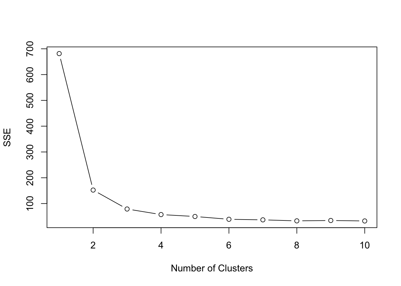

We can see that k = 3 is a good pick and actually approximates the number of species available in the iris dataset.

Silhouette coefficient

To calculate the Silhouette coefficient we have to install and load the library cluster:

# Assuming cluster library is installed with: install.packages('cluster')
library(cluster)
silhouette = silhouette(clustering$cluster, dist(data))
plot(silhouette)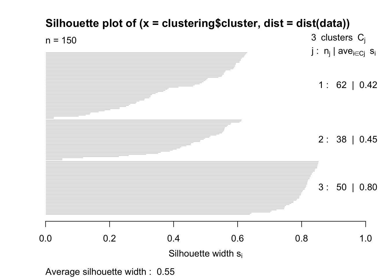

The closer to 1 the better.